重采样方法旨在从训练数据集中添加或删除示例,以更改类别分布。
一旦类分布更加平衡,标准的机器学习分类算法套件,就可以成功地拟合在转换后的数据集上。
过采样方法在少数类中复制或创建新的合成示例,而欠采样方法则在多数类中删除或合并示例。两种类型的重采样在单独使用时都可以有效,但是当两种方法一起使用时可能更有效。
在本教程中,您将发现如何结合使用过采样和欠采样技术进行不平衡分类。
完成本教程后,您将知道:
- 如何定义一个应用于训练数据集或评估分类器模型时的,过采样和欠采样方法的序列。
- 如何手动组合过采样和欠采样方法,以实现不平衡分类。
- 如何使用预定义和性能良好的重采样方法组合,进行不平衡分类。
教程概述
本教程分为四个部分:
- 二进制测试问题和决策树模型
- 不平衡学习的库(Imbalanced-Learn Library)
- 手动组合过采样和欠采样方法
- 手动组合随机过采样和欠采样
- 手动结合SMOTE和随机欠采样
- 使用预定义的重采样方法组合
- SMOTE和Tomek链接的组合欠采样
- SMOTE和编辑最近邻居(ENN)欠采样的组合
二进制测试问题和决策树模型
在深入研究过采样和欠采样方法的组合之前,让我们定义一个综合数据集和模型。
我们可以使用scikit-learn库中的make_classification()函数定义一个合成的二进制分类数据集。
例如,我们可以创建具有两个输入变量的,1:100类分布的10,000个示例,如下所示:
1
2
3
# define dataset
X, y = make_classification(n_samples=10000, n_features=2, n_redundant=0,
	n_clusters_per_class=1, weights=[0.99], flip_y=0, random_state=1)
然后,我们可以通过scatter()Matplotlib函数创建数据集的散点图,以了解每个类中示例的空间关系及其不平衡。
1
2
3
4
5
6
# scatter plot of examples by class label
for label, _ in counter.items():
	row_ix = where(y == label)[0]
	pyplot.scatter(X[row_ix, 0], X[row_ix, 1], label=str(label))
pyplot.legend()
pyplot.show()
结合在一起,下面列出了创建不平衡分类数据集,并绘制图例的完整示例。
1
2
3
4
5
6
7
8
9
10
11
12
13
14
15
16
17
# Generate and plot a synthetic imbalanced classification dataset
from collections import Counter
from sklearn.datasets import make_classification
from matplotlib import pyplot
from numpy import where
# define dataset
X, y = make_classification(n_samples=10000, n_features=2, n_redundant=0,
	n_clusters_per_class=1, weights=[0.99], flip_y=0, random_state=1)
# summarize class distribution
counter = Counter(y)
print(counter)
# scatter plot of examples by class label
for label, _ in counter.items():
	row_ix = where(y == label)[0]
	pyplot.scatter(X[row_ix, 0], X[row_ix, 1], label=str(label))
pyplot.legend()
pyplot.show()
首先运行示例以总结类的分布,显示出大约1:100的类分布,其中约10,000个示例的类为0,而100个类的类为1。
1
Counter({0: 9900, 1: 100})
接下来,创建一个散点图,显示数据集中的所有示例。我们可以看到大量的0类(蓝色)示例和少量1类(橙色)示例。
我们还可以看到,与类1的一些示例明显重叠的一些示例,同时属于类0的部分的要素空间内。
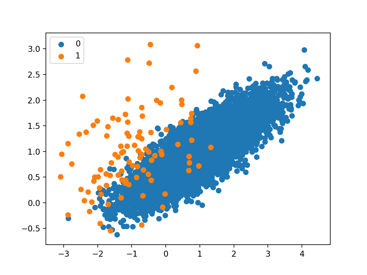 图说:不平衡分类数据集的散点图我们可以在此数据集上拟合DecisionTreeClassifier模型。这是一个很好的测试模型,因为它对训练数据集中的分类分布敏感。
1
2
# define model
model = DecisionTreeClassifier()
我们可以使用重复三次,并具有10折的k折交叉验证来评估模型。
曲线下的ROC面积(AUC)度量可用于估计模型的性能。虽然它确实正确显示了模型性能的相对改进,但对于严重不平衡的数据集可能是乐观的。
1
2
3
4
5
6
7
8
9
10
11
12
13
14
15
16
17
# evaluates a decision tree model on the imbalanced dataset
from numpy import mean
from sklearn.datasets import make_classification
from sklearn.tree import DecisionTreeClassifier
from sklearn.model_selection import cross_val_score
from sklearn.model_selection import RepeatedStratifiedKFold
# generate 2 class dataset
X, y = make_classification(n_samples=10000, n_features=2, n_redundant=0,
	n_clusters_per_class=1, weights=[0.99], flip_y=0, random_state=1)
# define model
model = DecisionTreeClassifier()
# define evaluation procedure
cv = RepeatedStratifiedKFold(n_splits=10, n_repeats=3, random_state=1)
# evaluate model
scores = cross_val_score(model, X, y, scoring='roc_auc', cv=cv, n_jobs=-1)
# summarize performance
print('Mean ROC AUC: %.3f' % mean(scores))
运行示例将报告,数据集上决策树模型,在三次重复10倍交叉验证中的平均ROC AUC(例如,在30种不同模型评估中的平均值)。
鉴于学习算法和评估程序的随机性,您的具体结果会有所不同。尝试运行该示例几次。
在此示例中,您可以看到该模型的ROC AUC约为0.76。这提供了该数据集的基线,我们可以用来比较训练数据集上,过采样方法和欠采样方法的不同组合。
1
Mean ROC AUC: 0.762
现在我们有了测试问题,模型和测试工具,让我们看一下过采样和欠采样方法的手动组合。
不平衡学习库
在这些示例中,我们将使用不平衡学习Python库,可以通过pip如下安装:
sudo pip install imbalanced-learn
您可以通过打印已安装的库的版本,来确认安装成功:
1
2
3
# check version number
import imblearn
print(imblearn.__version__)
运行示例将打印已安装库的版本号;例如:
1
0.5.0
手动组合过采样和欠采样方法
学习不平衡的Python库提供了一系列重采样技术,以及Pipeline类,可用于创建组合的重采样方法序列,以应用于数据集。
我们可以使用Pipeline构造一系列过采样和欠采样技术以应用于数据集。例如:
1
2
3
4
5
# define resampling
over =
under =
# define pipeline
pipeline = Pipeline(steps=[('o', over), ('u', under)])
该Pipeline首先将过采样技术应用于数据集,然后在返回最终结果之前,将欠采样应用于已通过过采样转换的输出集上。它允许将转换按顺序堆叠或应用到数据集。
然后可以使用pipeline来转换数据集。例如:
1
2
# fit and apply the pipeline
X_resampled, y_resampled = pipeline.fit_resample(X, y)
或者,可以将模型添加为pipeline中的最后一步。
这允许将pipeline视为模型。当它拟合在训练数据集时,首先将变换应用于训练数据集,然后将变换后的数据集提供给模型,以便可以进行拟合。
1
2
3
4
5
6
7
# define model
model =
# define resampling
over =
under =
# define pipeline
pipeline = Pipeline(steps=[('o', over), ('u', under), ('m', model)])
回想一下,重采样仅应用于训练数据集,而不是测试数据集。
当用于k折交叉验证时,将整个变换和拟合序列应用于由交叉验证折组成的每个训练数据集。这很重要,因为变换和拟合都在不了解预留数据集的情况下执行,从而避免了数据泄漏。例如:
1
2
3
4
# define evaluation procedure
cv = RepeatedStratifiedKFold(n_splits=10, n_repeats=3, random_state=1)
# evaluate model
scores = cross_val_score(pipeline, X, y, scoring='roc_auc', cv=cv, n_jobs=-1)
现在我们知道了如何手动组合重采样方法,下面让我们看两个示例。
手动组合随机过采样和欠采样
结合重采样技术的一个很好的起点,是从随机或幼稚的方法开始。
尽管它们很简单,并且在单独应用时通常无效,但结合使用它们可能会很有效。
随机过采样涉及在少数类别中随机复制示例,而随机欠采样涉及从多数类中随机删除示例。
由于这两个变换是在单独的类上执行的,因此将它们应用于训练数据集的顺序无关紧要。
下面的示例定义了一个pipeline,该pipeline首先将少数群体的样本过采样到多数群体的10%,然后将多数类别欠采样到少数群体的50%,然后拟合决策树模型。
1
2
3
4
5
6
7
# define model
model = DecisionTreeClassifier()
# define resampling
over = RandomOverSampler(sampling_strategy=0.1)
under = RandomUnderSampler(sampling_strategy=0.5)
# define pipeline
pipeline = Pipeline(steps=[('o', over), ('u', under), ('m', model)])
下面列出了,在2进制问题上,评估此组合的完整示例。
1
2
3
4
5
6
7
8
9
10
11
12
13
14
15
16
17
18
19
20
21
22
23
24
25
# combination of random oversampling and undersampling for imbalanced classification
from numpy import mean
from sklearn.datasets import make_classification
from sklearn.model_selection import cross_val_score
from sklearn.model_selection import RepeatedStratifiedKFold
from sklearn.tree import DecisionTreeClassifier
from imblearn.pipeline import Pipeline
from imblearn.over_sampling import RandomOverSampler
from imblearn.under_sampling import RandomUnderSampler
# generate dataset
X, y = make_classification(n_samples=10000, n_features=2, n_redundant=0,
	n_clusters_per_class=1, weights=[0.99], flip_y=0, random_state=1)
# define model
model = DecisionTreeClassifier()
# define resampling
over = RandomOverSampler(sampling_strategy=0.1)
under = RandomUnderSampler(sampling_strategy=0.5)
# define pipeline
pipeline = Pipeline(steps=[('o', over), ('u', under), ('m', model)])
# define evaluation procedure
cv = RepeatedStratifiedKFold(n_splits=10, n_repeats=3, random_state=1)
# evaluate model
scores = cross_val_score(pipeline, X, y, scoring='roc_auc', cv=cv, n_jobs=-1)
# summarize performance
print('Mean ROC AUC: %.3f' % mean(scores))
通过运行示例,可以评估转换系统和模型,并将性能总结为平均ROC AUC。
由于学习算法,重采样算法和评估程序的随机性,您的具体结果会有所不同。尝试运行该示例几次。
在这种情况下,我们可以看到ROC AUC性能从0.76适度提升,没有任何变换,随机过采样和欠采样大约达到0.81。
1
Mean ROC AUC: 0.814
手动结合SMOTE和随机欠采样
我们不限于使用随机重采样方法。
也许最流行的过采样方法是合成少数类过采样技术,简称SMOTE。
SMOTE的工作方式是选择特征空间中较近的示例,在特征空间中的示例之间绘制一条线,并沿着该线绘制一个新样本作为点。
该技术的作者建议在少数类别上使用SMOTE,然后在多数类别上使用欠采样技术。
“SMOTE和欠采样的组合比纯欠采样性能更好。”
— SMOTE:综合少数类过采样技术,2011年。
我们可以将SMOTE与RandomUnderSampler结合使用。同样,这些过程的应用顺序并不重要,因为它们是在训练数据集的不同子集上执行的。
下面的pipeline实现了这种组合,首先应用SMOTE,将少数类别的分布提高到多数类别的10%,然后使用RandomUnderSampler将多数类别的比例降低到少数类别的50%,然后再安装DecisionTreeClassifier。
1
2
3
4
5
6
# define model
model = DecisionTreeClassifier()
# define pipeline
over = SMOTE(sampling_strategy=0.1)
under = RandomUnderSampler(sampling_strategy=0.5)
steps = [('o', over), ('u', under), ('m', model)]
下面的示例,在我们的不平衡二进制分类问题上评估了这种组合。
1
2
3
4
5
6
7
8
9
10
11
12
13
14
15
16
17
18
19
20
21
22
23
24
25
# combination of SMOTE and random undersampling for imbalanced classification
from numpy import mean
from sklearn.datasets import make_classification
from sklearn.model_selection import cross_val_score
from sklearn.model_selection import RepeatedStratifiedKFold
from sklearn.tree import DecisionTreeClassifier
from imblearn.pipeline import Pipeline
from imblearn.over_sampling import SMOTE
from imblearn.under_sampling import RandomUnderSampler
# generate dataset
X, y = make_classification(n_samples=10000, n_features=2, n_redundant=0,
	n_clusters_per_class=1, weights=[0.99], flip_y=0, random_state=1)
# define model
model = DecisionTreeClassifier()
# define pipeline
over = SMOTE(sampling_strategy=0.1)
under = RandomUnderSampler(sampling_strategy=0.5)
steps = [('o', over), ('u', under), ('m', model)]
pipeline = Pipeline(steps=steps)
# define evaluation procedure
cv = RepeatedStratifiedKFold(n_splits=10, n_repeats=3, random_state=1)
# evaluate model
scores = cross_val_score(pipeline, X, y, scoring='roc_auc', cv=cv, n_jobs=-1)
# summarize performance
print('Mean ROC AUC: %.3f' % mean(scores))
通过运行示例,可以评估转换系统和模型,并将性能总结为平均ROC AUC。
由于学习算法,重采样算法和评估程序的随机性,您的具体结果会有所不同。尝试运行该示例几次。
在这种情况下,我们可以看到ROC AUC性能的另一个列表,从大约0.81到大约0.83。
1
Mean ROC AUC: 0.833
使用预定义的重采样方法组合
过采样和欠采样相结合方法,已经证明有效了,且他们结合一起,可被认为重采样技术。
两个示例是SMOTE与Tomek Link欠采样组合,以及SMOTE与Edited Nearest Neighbor欠采样的组合。
学习不平衡的Python库直接为这两种组合提供了实现。让我们依次仔细研究每个对象。
SMOTE和Tomek链接的组合欠采样
SMOTE是一种过采样方法,可以在多数类别中综合新的合理示例。
Tomek链接,是指一种用于识别数据集中具有不同类别的最近邻居对的方法。删除这些对中的一个或两个示例(例如,多数类中的示例)会降低训练数据集中的决策边界的噪音或歧义。
Gustavo Batista等,在2003年题为“ 针对关键字的自动注释的平衡训练数据:一个案例研究 (Balancing Training Data for Automated Annotation of Keywords: a Case Study)”的论文中对这些方法进行了测试。
具体而言,首先使用SMOTE方法对少数类别进行过采样以达到平衡分布,然后从多数类别中识别并删除Tomek链接中的示例。
“在这项工作中,仅删除了参与Tomek链接的多数类实例,因为少数类实例被认为太少而无法丢弃。[…]在我们的工作中,由于人为地创建了少数派示例,且数据集已经被平衡,因此删除了构成Tomek链接的多数类和少数类示例。”
— 针对关键字的自动注释的平衡培训数据:一个案例研究,2003年。
事实表明,该组合可以减少误报,但会增加二进制分类任务的误报。
我们可以使用SMOTETomek类实现此组合。
1
2
# define resampling
resample = SMOTETomek()
可以通过“ smote ”“ smote ”“ smote ”参数设置SMOTE配置,并采用已配置的SMOTE实例。可以通过“ tomek”参数设置Tomek Links配置,并采用已配置的TomekLinks 对象。
默认设置是使数据集与SMOTE保持平衡,然后从所有类中删除Tomek链接。这是另一篇论文中使用的方法,该论文探索了这种组合,标题为“ 平衡机器学习训练数据的几种方法的行为研究”(“A Study of the Behavior of Several Methods for Balancing Machine Learning Training Data.”)。
…我们建议将Tomek链接应用于过采样的训练集,作为数据清理方法。因此,不仅删除构成Tomek链接的多数类示例,还删除了两个类中的示例。
— 平衡机器学习训练数据的几种方法的行为研究,2004年。
另种方法是,我们通过从多数类中删除链接,来配置组合。在2003年的论文中,这些链接被描述为,通过TomekLinks用“ sampling_strategy ”参数设置的示例,所特定的tomek,去仅仅欠采样多数 类; 例如:
1
2
# define resampling
resample = SMOTETomek(tomek=TomekLinks(sampling_strategy='majority'))
我们可以使用,决策树分类器在二进制分类问题评估的这种组合重采样策略。
下面列出了完整的示例。
1
2
3
4
5
6
7
8
9
10
11
12
13
14
15
16
17
18
19
20
21
22
23
24
# combined SMOTE and Tomek Links resampling for imbalanced classification
from numpy import mean
from sklearn.datasets import make_classification
from sklearn.model_selection import cross_val_score
from sklearn.model_selection import RepeatedStratifiedKFold
from imblearn.pipeline import Pipeline
from sklearn.tree import DecisionTreeClassifier
from imblearn.combine import SMOTETomek
from imblearn.under_sampling import TomekLinks
# generate dataset
X, y = make_classification(n_samples=10000, n_features=2, n_redundant=0,
	n_clusters_per_class=1, weights=[0.99], flip_y=0, random_state=1)
# define model
model = DecisionTreeClassifier()
# define resampling
resample = SMOTETomek(tomek=TomekLinks(sampling_strategy='majority'))
# define pipeline
pipeline = Pipeline(steps=[('r', resample), ('m', model)])
# define evaluation procedure
cv = RepeatedStratifiedKFold(n_splits=10, n_repeats=3, random_state=1)
# evaluate model
scores = cross_val_score(pipeline, X, y, scoring='roc_auc', cv=cv, n_jobs=-1)
# summarize performance
print('Mean ROC AUC: %.3f' % mean(scores))
通过运行示例,可以评估转换系统和模型,并将性能总结为平均ROC AUC。
由于学习算法,重采样算法和评估程序的随机性,您的具体结果会有所不同。尝试运行该示例几次。
在这种情况下,似乎此组合重采样策略对该数据集上的模型没有提供优势。
1
Mean ROC AUC: 0.815
SMOTE和ENN欠采样的组合
SMOTE可能是最流行的过采样技术,并且可以与许多不同的欠采样技术结合使用。
另一种非常流行的欠采样方法是“编辑最近邻”或“ ENN”规则。该规则涉及使用k = 3最近邻居来定位数据集中分类错误的, 且随后被删除的那些示例。它可以应用于所有类,也可以应用于多数类中的那些示例。
Gustavo Batista等,对比其2004年“ 平衡机器学习训练数据的几种方法的行为研究 ”中使用的隔离方法,探索了过采样和欠采样方法的许多组合。
包括以下组合:
- CNN+ Tomek链接
- SMOTE + Tomek链接
- SMOTE +ENN
关于最后的组合,作者评论说,ENM比Tomek Links在降低大多数类别的采样方面更具侵略性,提供了更深入的清理。他们应用了该方法,从多数和少数类别中删除了示例。
…ENN用于从两个类中删除示例。因此,任何被其三个最近邻居错误分类的示例都将从训练集中删除。
— 平衡机器学习训练数据的几种方法的行为研究,2004年。
这可以通过不平衡学习库中的SMOTEENN类实现。
1
2
# define resampling
resample = SMOTEENN()
SMOTE配置可以通过1
smote
我们可以改变ENN,使其仅从多数类,通过设置enn参数的说法为一个EditedNearestNeighbours示例(该示例有着sampling_strategy参数)从而设置多数类”。
1
2
# define resampling
resample = SMOTEENN(enn=EditedNearestNeighbours(sampling_strategy='majority'))
我们可以评估默认策略(在所有类中编辑示例),并使用决策树分类器对不平衡数据集进行评估。
下面列出了完整的示例。
1
2
3
4
5
6
7
8
9
10
11
12
13
14
15
16
17
18
19
20
21
22
23
# combined SMOTE and Edited Nearest Neighbors resampling for imbalanced classification
from numpy import mean
from sklearn.datasets import make_classification
from sklearn.model_selection import cross_val_score
from sklearn.model_selection import RepeatedStratifiedKFold
from imblearn.pipeline import Pipeline
from sklearn.tree import DecisionTreeClassifier
from imblearn.combine import SMOTEENN
# generate dataset
X, y = make_classification(n_samples=10000, n_features=2, n_redundant=0,
	n_clusters_per_class=1, weights=[0.99], flip_y=0, random_state=1)
# define model
model = DecisionTreeClassifier()
# define resampling
resample = SMOTEENN()
# define pipeline
pipeline = Pipeline(steps=[('r', resample), ('m', model)])
# define evaluation procedure
cv = RepeatedStratifiedKFold(n_splits=10, n_repeats=3, random_state=1)
# evaluate model
scores = cross_val_score(pipeline, X, y, scoring='roc_auc', cv=cv, n_jobs=-1)
# summarize performance
print('Mean ROC AUC: %.3f' % mean(scores))
通过运行示例,可以评估转换系统和模型,并将性能总结为平均ROC AUC。
由于学习算法,重采样算法和评估程序的随机性,您的具体结果会有所不同。尝试运行该示例几次。
在这种情况下,通过随机欠采样方法,我们发现与SMOTE相比,性能会进一步提高,从大约0.81提高到大约0.85。
1
Mean ROC AUC: 0.856
该结果表明,编辑过采样的少数类别,可能也是一个很容易被忽略,但很重要的考虑因素。
这与2004年论文中的发现相同,作者发现使用Tomek Links的SMOTE和使用ENN的SMOTE在一系列数据集上表现良好。
我们的结果表明,特别是对于很少有阳性(少数)实例的数据集,总体而言,过采样方法以及Smote + Tomek和Smote + ENN(本工作中提出的两种方法),在实践中提供了很好的结果。
— 平衡机器学习训练数据的几种方法行为的研究,2004年。
- 编译:Florence Wong – AICUG
- 原文链接:https://zhuanlan.zhihu.com/p/159080497